Variable features
The dependent variable hypothesized in the article is the number of
dog bite incidents per zipcode. The predictor variables include the year
and month of the incident, characteristics of the dog, and the area
where the incident occurred. The year is measured as an interval-level
variable, with values from 1 (corresponding to 2015) to 7 (corresponding
to 2021). The area of the incident is divided into variables ranging
from 1 to 5, representing the five boroughs of New York City. The gender
of the dog is a binary variable, with 1 indicating female and 2
indicating male. Similarly, the sterilization status of the dog is also
a binary variable, with 0 indicating unsterilized and 1 indicating
sterilized.
data <- data.frame(
  `Variable` = c("dog_bite_incidents", "year", "month", "gender", "spay_neuter", "borough"),
  `Range` = c(
    "$\\mathbb{N}$",
    "$\\{1, 2, 3, 4, 5, 6, 7\\}$",
    "$\\{1, 2, 3, 4, 5, 6, 7, 8, 9, 10, 11, 12\\}$",
    "$\\{1, 2\\}$",
    "$\\{0, 1\\}$",
    "$\\{1, 2, 3, 4, 5\\}$"
  )
)

knitr::kable(data, format = "pipe", align = "l", caption = "Variable Implications")
Variable Implications
| dog_bite_incidents |
\(\mathbb{N}\) |
| year |
\(\{1, 2, 3, 4, 5, 6,
7\}\) |
| month |
\(\{1, 2, 3, 4, 5, 6, 7, 8,
9, 10, 11, 12\}\) |
| gender |
\(\{1, 2\}\) |
| spay_neuter |
\(\{0, 1\}\) |
| borough |
\(\{1, 2, 3, 4,
5\}\) |
Negative Binomial Regression Analysis
To measure the combined effects of year, dog background
characteristics (i.e., gender and whether neutered) and the Borough they
belong to on the incidence of dog bites, we first conduct a negative
binomial regression analysis using records of dog bite incidents in New
York.
The negative binomial regression model is a type of count model
designed for dependent variables that can only take non-negative integer
values. From the Spatial Correlations section, the study area meets the
three prerequisites for negative binomial regression: the dog bite
incidents are not independent, exhibiting spatial clustering; the
dependent variable shows overdispersion; and the frequency of dog bite
incidents is sufficiently low. Let the dependent variable follows a
negative binomial distribution. The model equation is as follows:
\[\ln ({\hat y_i}) = {\beta _0} + {\beta
_1}{X_{i1}} + {\beta _2}{X_{i2}} + \cdots {\beta _m}{X_{im}} +
\xi\]
Here, \({y_i}\) represents the
frequency of dog bite incidents within a year, \({\beta _m}\) is the coefficient, \(X_m\) are the explanatory variables, and
\(\xi\) represents the heterogeneity
across observations.
In negative binomial regression, where the conditional expectation
\(E(Y|X) = e^{\beta_0 + \beta_1 X_{i1} +
\beta_2 X_{i2} + \cdots + \beta_m X_{im}}\), the interpretation
of the model’s coefficients is as follows: when the explanatory variable
\({X_k}\) increases by one unit, the
average occurrence rate of dog bite incidents becomes \({e^{{\beta _k}}}\) times what it was
originally.
\[
\frac{E(Y|X^*)}{E(Y|X)} = \frac{e^{\beta_0 + \beta_1 X_{i1} + \cdots +
\beta_k (X_{ik} + 1) + \cdots + \beta_m X_{im}}}{e^{\beta_0 + \beta_1
X_{i1} + \cdots + \beta_k X_{ik} + \cdots + \beta_m X_{im}}} =
e^{\beta_k}
\]
Regularized Model (Lasso)
Initially, the paper employs Lasso regression on five primary
variables, aiming to use regularization to reduce the number of
variables in the model and thus avoid overfitting.
# lasso

x = model.matrix(bite_count ~ year + month + gender + spay_neuter + borough, data = bites_by_group)
y = bites_by_group |> pull(bite_count)

cv_model = cv.glmnet(x, y, family = "poisson", alpha = 1)  # Lasso:alpha = 1

cv_results <- with(cv_model,
  data.frame(
  log_lambda = log(lambda),
  mean_mse = cvm,
  lower_mse = cvlo,
  upper_mse = cvup
))

best_lambda <- cv_model$lambda.min
log_best_lambda <- log(best_lambda)
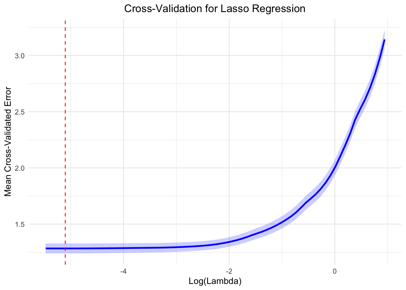
\(\lambda\) is the regularization
parameter in Lasso regression, controlling variable selection and the
sparsity of the model. Finding the optimal \(\lambda\) value is crucial as it balances
model complexity and predictive performance. The ideal \(\lambda\) value, derived from
cross-validation, minimizes model error. For this study, the optimal
\(\lambda\) has been determined to be
0.005529689.
ggplot(cv_results, aes(x = log_lambda, y = mean_mse)) +
  geom_line(color = "blue", size = 1) +
  geom_ribbon(aes(ymin = lower_mse, ymax = upper_mse), alpha = 0.2, fill = "blue") +
  geom_vline(xintercept = log_best_lambda, linetype = "dashed", color = "red") +
  labs(
    title = "Cross-Validation for Lasso Regression",
    x = "Log(Lambda)",
    y = "Mean Cross-Validated Error"
  ) +
  theme_minimal() +
  theme(plot.title = element_text(hjust = 0.5))

lasso_coefficients <- coef(cv_model, s = "lambda.min")

lasso_coefficients_df <- as.data.frame(as.matrix(lasso_coefficients)) %>%
  rownames_to_column("Variable") %>%
  rename(Coefficient = 1) %>%
  filter(Coefficient != 0)

kable(
  lasso_coefficients_df,
  col.names = c("Term", "Coefficient"),
  caption = "Cross-Validation Results for Lasso Regression",
  align = "c",
  digits = 4
) |>
  kable_styling(
    bootstrap_options = c("striped", "hover", "condensed", "responsive"),
    full_width = TRUE
  ) |>
  scroll_box(height = "300px")
Cross-Validation Results for Lasso Regression
|
Term
|
Coefficient
|
|
X.Intercept.
|
1.1070
|
|
X.Intercept..1
|
0.0000
|
|
year2016
|
0.0589
|
|
year2017
|
0.1471
|
|
year2018
|
0.0711
|
|
year2019
|
0.0949
|
|
year2020
|
-0.2819
|
|
year2021
|
-0.2845
|
|
month2
|
-0.0167
|
|
month3
|
0.0000
|
|
month4
|
0.1036
|
|
month5
|
0.1568
|
|
month6
|
0.2253
|
|
month7
|
0.1832
|
|
month8
|
0.2052
|
|
month9
|
0.1186
|
|
month10
|
0.0678
|
|
month11
|
0.0588
|
|
month12
|
-0.0010
|
|
genderM
|
0.8880
|
|
spay_neuterNeutered
|
-0.1034
|
|
boroughBrooklyn
|
0.2990
|
|
boroughManhattan
|
0.2263
|
|
boroughQueens
|
0.4942
|
|
boroughStaten.Island
|
-0.5573
|
In summary, the Lasso regression model selected the following
variables:
- Time factor:
year and month
- Individual characteristics:
gender and
spay_neuter
- Regional characteristics:
borough
Therefore, these variables need to be included in the subsequent
negative binomial regression analysis.
Main effects model
After employing Lasso regression for feature selection, the study
identified several key variables that influence the occurrence of dog
bite incidents. These variables include the year,
month, gender, spay_neuter, and
borough. These factors will be incorporated into a negative
binomial generalized linear model (glm.nb) to predict the
number of bite incidents.
Results
The results of the main effects model fitting are presented in the
following table.
The dispersion parameter, \(\theta =
25.18\), indicates that the data exhibits overdispersion, meaning
the variance is much larger than the mean. This justifies the use of the
negative binomial regression model over a Poisson regression.
The deviance of the null model (a model with no predictors, only the
intercept) is \(3914.5\). This
represents the deviance of the fitted model with predictors included is
\(1549.7\). The significant reduction
in deviance indicates that the included predictors substantially improve
model fit.
kable(
  model_summary,
  col.names = c("Term", "Estimate", "SE", "Statistic", "P-value", "Significance"),
  caption = "Summary of Negative Binomial Regression Results"
) %>%
  kable_styling(bootstrap_options = c("striped", "hover", "condensed"), full_width = TRUE) %>%
  scroll_box(height = "400px")
Summary of Negative Binomial Regression Results
|
Term
|
Estimate
|
SE
|
Statistic
|
P-value
|
Significance
|
|
(Intercept)
|
1.0819840
|
0.0594554
|
18.1982535
|
0.0000000
|
***
|
|
year2016
|
0.0697408
|
0.0415739
|
1.6775135
|
0.0934421
|
|
|
year2017
|
0.1535577
|
0.0409067
|
3.7538482
|
0.0001741
|
***
|
|
year2018
|
0.0752355
|
0.0415347
|
1.8113915
|
0.0700803
|
|
|
year2019
|
0.0942075
|
0.0413851
|
2.2763627
|
0.0228243
|
|
|
year2020
|
-0.2791303
|
0.0454262
|
-6.1446913
|
0.0000000
|
***
|
|
year2021
|
-0.2870956
|
0.0458795
|
-6.2576004
|
0.0000000
|
***
|
|
month2
|
0.0025297
|
0.0587213
|
0.0430799
|
0.9656378
|
|
|
month3
|
0.0299763
|
0.0582325
|
0.5147697
|
0.6067140
|
|
|
month4
|
0.1274838
|
0.0571182
|
2.2319298
|
0.0256196
|
|
|
month5
|
0.1807138
|
0.0565828
|
3.1937937
|
0.0014042
|
**
|
|
month6
|
0.2447988
|
0.0559689
|
4.3738342
|
0.0000122
|
***
|
|
month7
|
0.2019422
|
0.0565467
|
3.5712485
|
0.0003553
|
***
|
|
month8
|
0.2276408
|
0.0563495
|
4.0397994
|
0.0000535
|
***
|
|
month9
|
0.1429531
|
0.0571015
|
2.5034925
|
0.0122974
|
|
|
month10
|
0.0912030
|
0.0577714
|
1.5786867
|
0.1144079
|
|
|
month11
|
0.0888914
|
0.0577247
|
1.5399200
|
0.1235799
|
|
|
month12
|
0.0185023
|
0.0588556
|
0.3143674
|
0.7532420
|
|
|
genderM
|
0.8851206
|
0.0245208
|
36.0966638
|
0.0000000
|
***
|
|
spay_neuterNeutered
|
-0.1122779
|
0.0228317
|
-4.9176281
|
0.0000009
|
***
|
|
boroughBrooklyn
|
0.3051114
|
0.0361136
|
8.4486684
|
0.0000000
|
***
|
|
boroughManhattan
|
0.2376617
|
0.0365134
|
6.5088955
|
0.0000000
|
***
|
|
boroughQueens
|
0.4981809
|
0.0349699
|
14.2459962
|
0.0000000
|
***
|
|
boroughStaten Island
|
-0.5517553
|
0.0446767
|
-12.3499477
|
0.0000000
|
***
|
Year: Some years (e.g., 2017, 2019) show statistically
significant coefficients, suggesting that the number of bite incidents
varies significantly across years. year2021 (Coefficient =
-0.28710, p < 0.001) indicates a significant
decrease in bite counts compared to year2015.
Month: Some months show no significant effects on bite
counts (e.g., month2: p = 0.97; month3: p = 0.61). Several months (e.g.,
May, June, August) have significant coefficients, indicating seasonality
in bite incidents.
Gender: Male dogs (genderM) are associated with a
significantly higher bite count, as indicated by the large positive
coefficient.
Spay/Neuter: Neutered dogs are associated with a lower
bite count, with a statistically significant negative coefficient.
Boroughs: Bite counts vary across boroughs, with Staten
Island showing a significant negative association compared to the
reference borough.
From the coefficient of fitting results, this study draws the
following conclusions:
Different years have significantly impacted bite counts,
particularly after 2020, where a notable reduction in incidents was
observed. This might reflect external factors, such as the COVID-19
pandemic.
Monthly effects highlight significant seasonal variation, with
summer months (e.g., June) showing higher bite counts.
Males are significantly more likely to be involved in bite
incidents than females.
Neutered animals have significantly lower bite risks compared to
non-neutered ones.
Brooklyn has significantly higher bite counts, while Staten
Island has significantly fewer bites compared to Bronx. These
differences might reflect variations in dog management policies,
population density, or dog ownership practices across regions.
Evaluation
After obtaining the fitted results, it is crucial to perform a
multicollinearity test on the model to ensure the reliability of the
regression coefficients. Multicollinearity can severely affect the
interpretability of the model and can lead to overinflated standard
errors, making it difficult to discern the true effect of each
predictor.
vif_results <- vif(model) %>%
  as.data.frame() %>%
  rownames_to_column("Predictor") %>%
  rename(
    GVIF = GVIF,
    DF = Df,
    `GVIF^(1/(2*DF))` = `GVIF^(1/(2*Df))`
  )

kable(
  vif_results,
  col.names = c("Predictor", "GVIF", "DF", "Scaled GVIF"),
  caption = "Multicollinearity Check (GVIF)"
) |>
  kable_styling(bootstrap_options = c("striped", "hover", "condensed"), full_width = TRUE)
Multicollinearity Check (GVIF)
|
Predictor
|
GVIF
|
DF
|
Scaled GVIF
|
|
year
|
1.004775
|
6
|
1.000397
|
|
month
|
1.002312
|
11
|
1.000105
|
|
gender
|
1.003175
|
1
|
1.001586
|
|
spay_neuter
|
1.001316
|
1
|
1.000658
|
|
borough
|
1.005447
|
4
|
1.000679
|
Generalized Variance Inflation Factor (GVIF) measures the
multicollinearity in the regression model. A GVIF value greater than 10
generally indicates a high multicollinearity issue. All GVIF values are
close to 1, suggesting no significant multicollinearity.
Scaled GVIF adjusts GVIF based on the degrees of freedom to make it
comparable across variables. It is defined as \(GVIF^{(1/(2*Df))}\). As shown in the table
above, the GVIF and scaled GVIF are all close to 1, indicating that
there is no significant multicollinearity in the final model.
As shown in the table above, results does not exhibit
multicollinearity among the predictors, as all GVIF values and their
scaled counterparts are well below the threshold of concern (commonly 10
or higher). This indicates that all predictors can be reliably used in
regression model without the risk of biased coefficients caused by
multicollinearity.
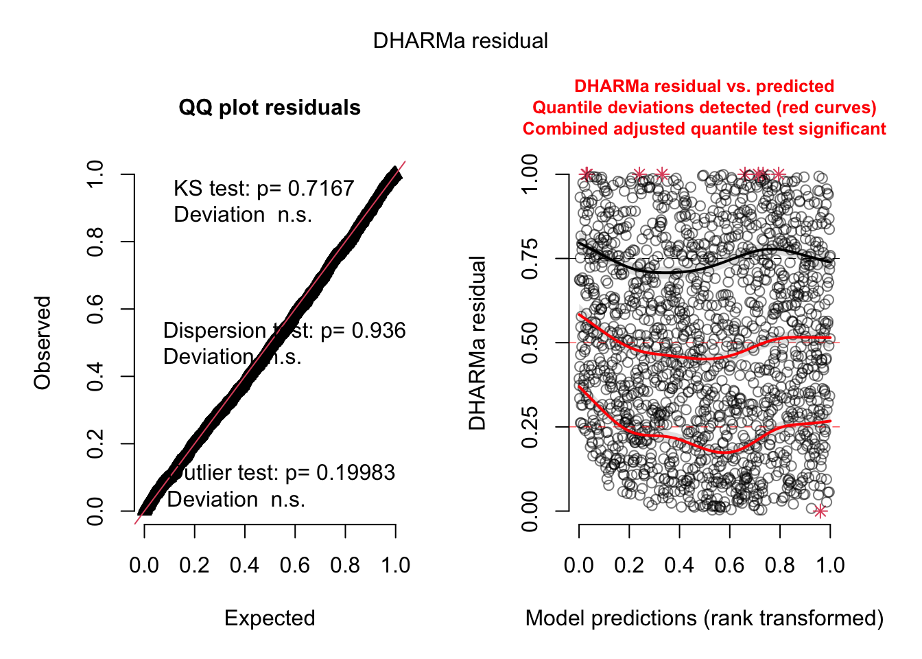
residuals_sim = simulateResiduals(model)
plot(residuals_sim)

Q-Q Plot:
- KS Test p-value (0.7167): Indicates that the residuals do not
significantly deviate from a uniform distribution. This suggests that
the model residuals are well-behaved.
- Dispersion Test p-value (0.936): Suggests there is no significant
over- or under-dispersion in the model, further supporting the
appropriateness of the negative binomial distribution.
- Outlier Test p-value (0.19983): Shows that there are no significant
outliers in the residuals, meaning that most predictions align with the
observed data.
The residuals closely follow the expected line, indicating a good fit
in terms of normality for the main effects-only model.
Residuals vs Predicted:
- The residuals appear to be well-distributed, with most points
clustering around the 0.5 quantile line.
- The red curves (quantile deviations) show minor deviations,
particularly near the tails (e.g., quantiles close to 0 and 1). However,
these deviations are not substantial enough to indicate severe model
misspecification.
- The presence of small red asterisks (*) at the upper quantiles
suggests slight issues with model fit in extreme predictions, but these
deviations are minor.
This shows some spread and potential systematic patterns, indicating
the main effects model might not fully capture the
variability in the data.
Model with interaction
To further increase the precision of the model fit, interaction terms
between variables were added.
Results
model_all_interactions <- glm.nb(
  formula = bite_count ~
    year + month + gender + spay_neuter + borough +
    year * month + year * gender + year * spay_neuter + year * borough +
    month * gender + month * spay_neuter + month * borough +
    gender * spay_neuter + gender * borough + spay_neuter * borough +
    year * month * gender + year * month * spay_neuter + year * month * borough +
    year * gender * spay_neuter + year * gender * borough + year * spay_neuter * borough +
    month * gender * spay_neuter + month * gender * borough + month * spay_neuter * borough +
    gender * spay_neuter * borough,
  data = bites_by_group
)

model_stepwise <- stepAIC(model_all_interactions, direction = "both")
After using stepwise reduction to simplify the model complexity, the
variables of final negative binomial regression model are as follow:
data <- data.frame(
  `Main Effect` = c("year", "month", "gender", "spay_neuter", "borough", " "),
  `Double Interaction Effect` = c(
    "year * spay_neuter",
    "year * borough",
    "month * spay_neuter",
    "gender * spay_neuter",
    "gender * borough",
    "spay_neuter * borough"
  )
)

knitr::kable(data, format = "pipe", align = "l", caption = "Final Negative Binomial Regression Model", escape = FALSE)
Final Negative Binomial Regression Model
| year |
year * spay_neuter |
| month |
year * borough |
| gender |
month * spay_neuter |
| spay_neuter |
gender * spay_neuter |
| borough |
gender * borough |
|
spay_neuter * borough |
The final model with interaction is detailed in the following table.
Firstly, the intercept is 3.83 with a p-value near zero, indicating that
the baseline level of the response variable (on a logarithmic scale) is
significant when other variables are not considered. For the main effect
variables, the years 2016, 2018, and 2019 show a significant increase in
the log change of event counts compared to 2015; male dogs, compared to
female dogs, exhibit stronger aggression, with a 10.59 times increase in
the incidence of dog bite events, calculated as with \(e^{2.36}\). The coefficient for neutering,
0.3960, indicates a significant reduction in the log count of bite
incidents for neutered dogs compared to unneutered dogs. Geographically,
the coefficients for Manhattan and Staten Island are 0.72 and 0.48,
respectively, showing significantly lower event counts compared to the
Bronx. Regarding interaction terms, the years 2018, 2020, and 2021 show
a significant reduction in interaction with the neutering status.
filter_model = glm.nb(bite_count ~ year + month + gender + spay_neuter +
    borough + year:spay_neuter + year:borough + month:spay_neuter +
    gender:spay_neuter + gender:borough + spay_neuter:borough,
    data = bites_by_group)

filter_model_summary <- tidy(filter_model, exponentiate = TRUE, conf.int = TRUE)

kable(
  filter_model_summary,
  caption = "Summary of Negative Binomial Regression (with interactions) Results"
) %>%
  kable_styling(bootstrap_options = c("striped", "hover", "condensed"), full_width = TRUE) %>%
  scroll_box(height = "400px")
Summary of Negative Binomial Regression (with interactions) Results
|
term
|
estimate
|
std.error
|
statistic
|
p.value
|
conf.low
|
conf.high
|
|
(Intercept)
|
3.8266218
|
0.0917147
|
14.6321455
|
0.0000000
|
3.1897224
|
4.5699845
|
|
year2016
|
1.3033610
|
0.0901036
|
2.9404628
|
0.0032772
|
1.0929752
|
1.5562867
|
|
year2017
|
1.1385007
|
0.0922903
|
1.4054815
|
0.1598781
|
0.9504021
|
1.3649459
|
|
year2018
|
1.3118411
|
0.0908169
|
2.9887793
|
0.0028009
|
1.0984502
|
1.5684738
|
|
year2019
|
1.3122458
|
0.0905443
|
3.0011837
|
0.0026893
|
1.0994102
|
1.5681645
|
|
year2020
|
0.8228914
|
0.1047046
|
-1.8617234
|
0.0626421
|
0.6693712
|
1.0093955
|
|
year2021
|
0.8059884
|
0.1072938
|
-2.0102369
|
0.0444061
|
0.6520723
|
0.9933690
|
|
month2
|
0.9729195
|
0.0695666
|
-0.3946429
|
0.6931064
|
0.8487826
|
1.1149947
|
|
month3
|
1.0105442
|
0.0684963
|
0.1531328
|
0.8782936
|
0.8835430
|
1.1557926
|
|
month4
|
0.9934017
|
0.0684907
|
-0.0966578
|
0.9229981
|
0.8685643
|
1.1361738
|
|
month5
|
1.0680211
|
0.0672828
|
0.9780735
|
0.3280380
|
0.9361209
|
1.2187538
|
|
month6
|
1.1690766
|
0.0657587
|
2.3755679
|
0.0175220
|
1.0278987
|
1.3302616
|
|
month7
|
1.2098715
|
0.0654067
|
2.9127615
|
0.0035825
|
1.0645334
|
1.3757713
|
|
month8
|
1.1509696
|
0.0664863
|
2.1147913
|
0.0344477
|
1.0104735
|
1.3114496
|
|
month9
|
1.0335144
|
0.0680631
|
0.4843299
|
0.6281517
|
0.9044289
|
1.1811049
|
|
month10
|
1.0959521
|
0.0673646
|
1.3601127
|
0.1737943
|
0.9604423
|
1.2508199
|
|
month11
|
1.0178300
|
0.0683075
|
0.2587259
|
0.7958467
|
0.8902585
|
1.1637148
|
|
month12
|
0.9873063
|
0.0689063
|
-0.1853956
|
0.8529188
|
0.8625001
|
1.1300826
|
|
genderM
|
2.3603576
|
0.0546184
|
15.7238806
|
0.0000000
|
2.1222253
|
2.6290269
|
|
spay_neuterNeutered
|
0.3960162
|
0.1090476
|
-8.4944592
|
0.0000000
|
0.3196063
|
0.4900996
|
|
boroughBrooklyn
|
1.1484679
|
0.1007295
|
1.3742626
|
0.1693602
|
0.9433984
|
1.4003372
|
|
boroughManhattan
|
0.7189159
|
0.1083180
|
-3.0466848
|
0.0023138
|
0.5815085
|
0.8892388
|
|
boroughQueens
|
1.0052349
|
0.1004848
|
0.0519610
|
0.9585598
|
0.8261307
|
1.2250977
|
|
boroughStaten Island
|
0.4792828
|
0.1295018
|
-5.6791829
|
0.0000000
|
0.3711956
|
0.6168309
|
|
year2016:spay_neuterNeutered
|
1.0612336
|
0.0738846
|
0.8043893
|
0.4211722
|
0.9181842
|
1.2266608
|
|
year2017:spay_neuterNeutered
|
1.1261719
|
0.0722120
|
1.6454912
|
0.0998686
|
0.9775818
|
1.2974768
|
|
year2018:spay_neuterNeutered
|
0.8361551
|
0.0738241
|
-2.4238853
|
0.0153555
|
0.7234554
|
0.9662810
|
|
year2019:spay_neuterNeutered
|
0.8999070
|
0.0732977
|
-1.4388429
|
0.1501950
|
0.7794484
|
1.0389210
|
|
year2020:spay_neuterNeutered
|
0.7093584
|
0.0832625
|
-4.1242377
|
0.0000372
|
0.6023798
|
0.8349059
|
|
year2021:spay_neuterNeutered
|
0.7033678
|
0.0842494
|
-4.1765924
|
0.0000296
|
0.5961124
|
0.8294237
|
|
year2016:boroughBrooklyn
|
0.6696158
|
0.1136113
|
-3.5300282
|
0.0004155
|
0.5356558
|
0.8362826
|
|
year2017:boroughBrooklyn
|
0.8016684
|
0.1146289
|
-1.9284860
|
0.0537947
|
0.6401252
|
1.0033867
|
|
year2018:boroughBrooklyn
|
0.6156245
|
0.1168101
|
-4.1530513
|
0.0000328
|
0.4893635
|
0.7736536
|
|
year2019:boroughBrooklyn
|
0.6430267
|
0.1158853
|
-3.8103961
|
0.0001387
|
0.5120816
|
0.8066385
|
|
year2020:boroughBrooklyn
|
0.9194226
|
0.1308903
|
-0.6418304
|
0.5209833
|
0.7116333
|
1.1889894
|
|
year2021:boroughBrooklyn
|
0.9169286
|
0.1340716
|
-0.6468607
|
0.5177221
|
0.7053947
|
1.1933845
|
|
year2016:boroughManhattan
|
0.7672008
|
0.1219690
|
-2.1727381
|
0.0298000
|
0.6038442
|
0.9741476
|
|
year2017:boroughManhattan
|
1.0056926
|
0.1214035
|
0.0467566
|
0.9627072
|
0.7926301
|
1.2758780
|
|
year2018:boroughManhattan
|
1.0764166
|
0.1200012
|
0.6136403
|
0.5394531
|
0.8507054
|
1.3618503
|
|
year2019:boroughManhattan
|
1.0374713
|
0.1197084
|
0.3072990
|
0.7586158
|
0.8203777
|
1.3117924
|
|
year2020:boroughManhattan
|
1.3188623
|
0.1365701
|
2.0265749
|
0.0427059
|
1.0096615
|
1.7248937
|
|
year2021:boroughManhattan
|
1.2422379
|
0.1397488
|
1.5521743
|
0.1206205
|
0.9452097
|
1.6350671
|
|
year2016:boroughQueens
|
0.8140961
|
0.1136471
|
-1.8097847
|
0.0703292
|
0.6512614
|
1.0169129
|
|
year2017:boroughQueens
|
1.0867730
|
0.1135860
|
0.7325963
|
0.4638047
|
0.8696893
|
1.3576659
|
|
year2018:boroughQueens
|
1.0448140
|
0.1131393
|
0.3874768
|
0.6984032
|
0.8367859
|
1.3040097
|
|
year2019:boroughQueens
|
1.0220010
|
0.1127442
|
0.1930255
|
0.8469390
|
0.8191320
|
1.2745219
|
|
year2020:boroughQueens
|
1.1261820
|
0.1306208
|
0.9097565
|
0.3629509
|
0.8722475
|
1.4557937
|
|
year2021:boroughQueens
|
1.2916043
|
0.1315466
|
1.9452047
|
0.0517504
|
0.9988859
|
1.6732506
|
|
year2016:boroughStaten Island
|
0.8644796
|
0.1431569
|
-1.0172580
|
0.3090307
|
0.6528959
|
1.1446386
|
|
year2017:boroughStaten Island
|
0.9866068
|
0.1425223
|
-0.0946074
|
0.9246267
|
0.7462658
|
1.3050651
|
|
year2018:boroughStaten Island
|
0.8321089
|
0.1483069
|
-1.2392683
|
0.2152461
|
0.6218356
|
1.1124636
|
|
year2019:boroughStaten Island
|
0.7854488
|
0.1468059
|
-1.6450292
|
0.0999638
|
0.5887784
|
1.0471310
|
|
year2020:boroughStaten Island
|
0.8911374
|
0.1789898
|
-0.6439284
|
0.5196219
|
0.6254889
|
1.2624986
|
|
year2021:boroughStaten Island
|
0.7210547
|
0.1929227
|
-1.6951883
|
0.0900397
|
0.4913490
|
1.0477969
|
|
month2:spay_neuterNeutered
|
1.0975279
|
0.1046014
|
0.8896655
|
0.3736455
|
0.8942084
|
1.3475758
|
|
month3:spay_neuterNeutered
|
1.0590365
|
0.1038588
|
0.5522843
|
0.5807536
|
0.8640731
|
1.2983755
|
|
month4:spay_neuterNeutered
|
1.3564416
|
0.1010573
|
3.0167522
|
0.0025550
|
1.1130392
|
1.6541988
|
|
month5:spay_neuterNeutered
|
1.3064944
|
0.0998785
|
2.6767279
|
0.0074345
|
1.0745154
|
1.5895806
|
|
month6:spay_neuterNeutered
|
1.2478170
|
0.0984299
|
2.2492726
|
0.0244952
|
1.0291517
|
1.5138497
|
|
month7:spay_neuterNeutered
|
1.0553692
|
0.0998428
|
0.5397557
|
0.5893656
|
0.8679186
|
1.2837758
|
|
month8:spay_neuterNeutered
|
1.2270280
|
0.0991555
|
2.0633748
|
0.0390770
|
1.0105739
|
1.4907576
|
|
month9:spay_neuterNeutered
|
1.2860456
|
0.1009214
|
2.4927527
|
0.0126757
|
1.0555295
|
1.5678926
|
|
month10:spay_neuterNeutered
|
1.0214410
|
0.1025915
|
0.2067852
|
0.8361776
|
0.8354704
|
1.2491730
|
|
month11:spay_neuterNeutered
|
1.1718216
|
0.1024908
|
1.5470612
|
0.1218485
|
0.9587419
|
1.4329166
|
|
month12:spay_neuterNeutered
|
1.0804447
|
0.1049678
|
0.7371092
|
0.4610559
|
0.8795844
|
1.3274456
|
|
genderM:spay_neuterNeutered
|
0.8800375
|
0.0453079
|
-2.8204976
|
0.0047949
|
0.8052402
|
0.9617512
|
|
genderM:boroughBrooklyn
|
1.1720073
|
0.0714328
|
2.2219198
|
0.0262887
|
1.0187251
|
1.3479804
|
|
genderM:boroughManhattan
|
1.1329946
|
0.0725463
|
1.7211669
|
0.0852205
|
0.9826828
|
1.3059767
|
|
genderM:boroughQueens
|
1.1693112
|
0.0684173
|
2.2861904
|
0.0222431
|
1.0222794
|
1.3367837
|
|
genderM:boroughStaten Island
|
0.9069992
|
0.0917203
|
-1.0642550
|
0.2872132
|
0.7582574
|
1.0864392
|
|
spay_neuterNeutered:boroughBrooklyn
|
2.4562537
|
0.0693940
|
12.9497913
|
0.0000000
|
2.1451226
|
2.8158263
|
|
spay_neuterNeutered:boroughManhattan
|
3.1397417
|
0.0704595
|
16.2382769
|
0.0000000
|
2.7364237
|
3.6070334
|
|
spay_neuterNeutered:boroughQueens
|
2.6530410
|
0.0670062
|
14.5614399
|
0.0000000
|
2.3279835
|
3.0273936
|
|
spay_neuterNeutered:boroughStaten Island
|
2.7436374
|
0.0868963
|
11.6148176
|
0.0000000
|
2.3149684
|
3.2546430
|
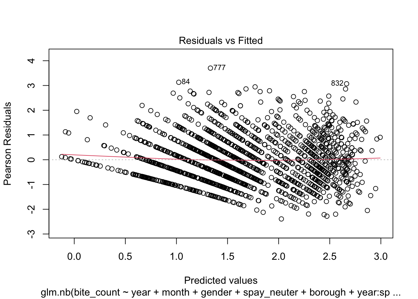
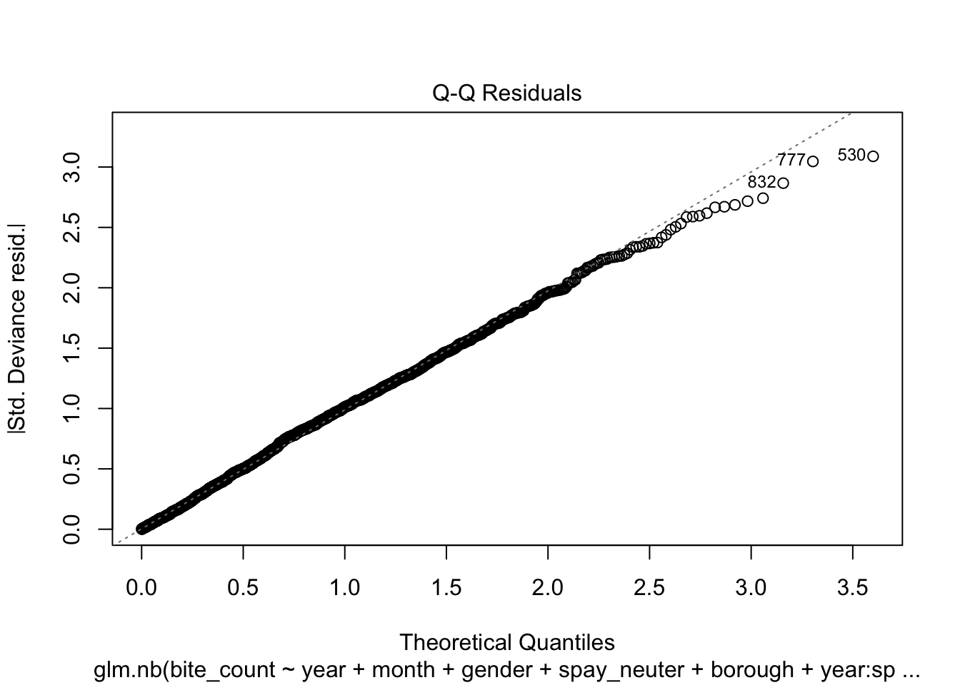
Evaluation
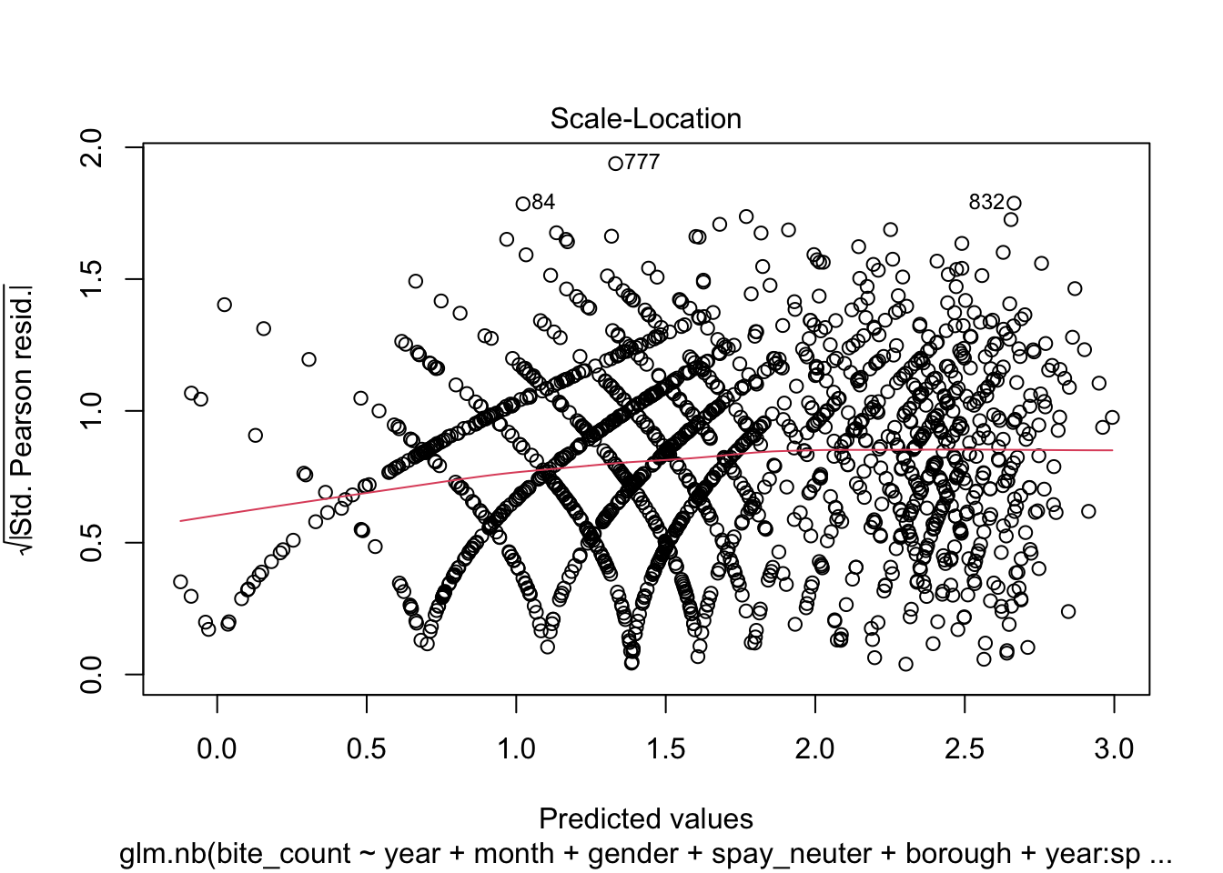
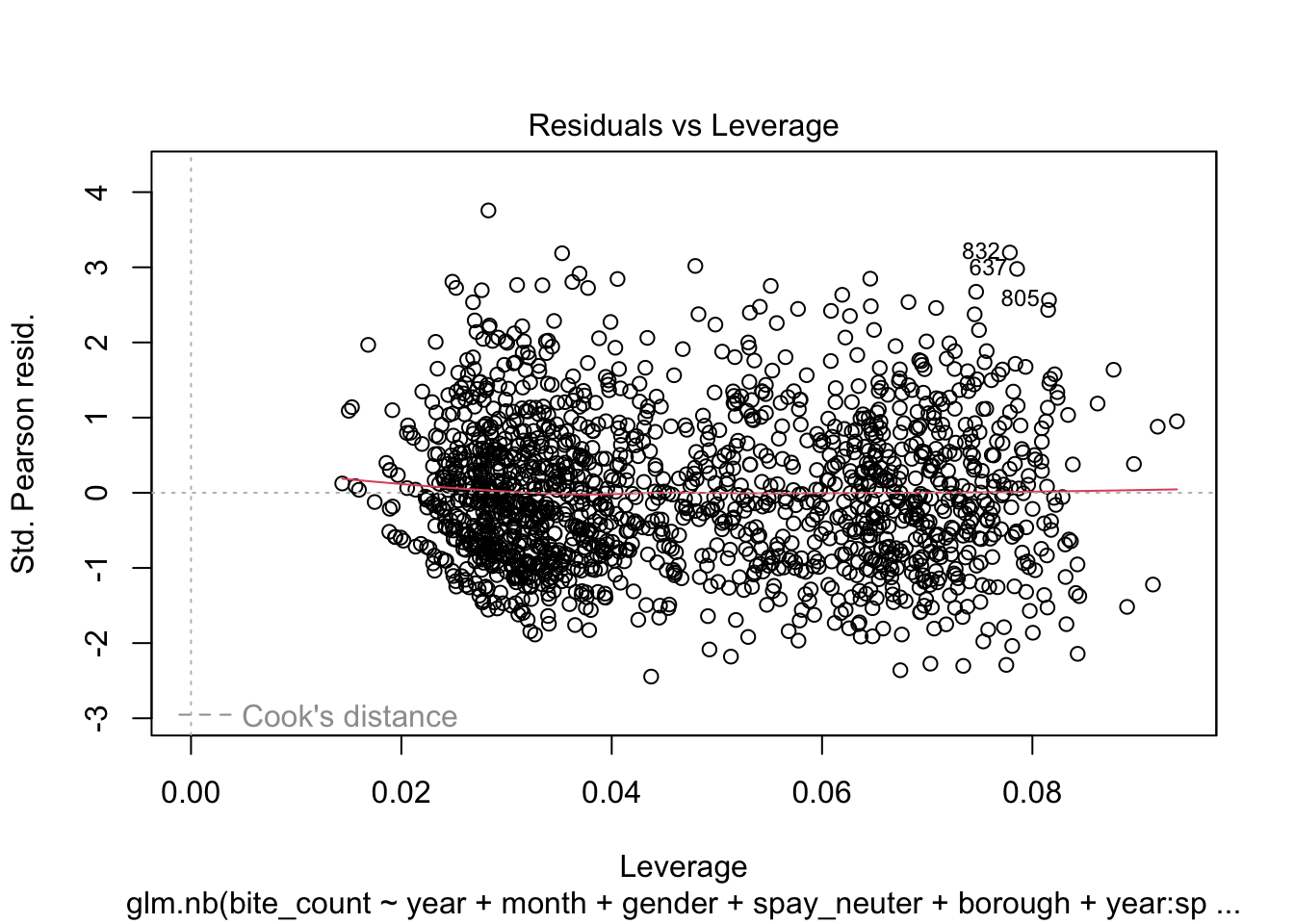
Additionally, the quality of the fitted model can be assessed through
residual analysis and diagnostics, as illustrated in the following four
plots.
- Residual vs. Fitted Plot:
This graph helps to detect non-linearity, unequal error variances,
and outliers. Ideally, the residuals should be randomly dispersed around
the horizontal axis, meaning the red dashed line (a smooth curve) should
be close to a horizontal straight line.
This plot is used to check whether the residuals conform to the
distribution assumed by the model.
This plot shows the spread of residuals versus fitted values and
helps to check for homoscedasticity (constant spread of residuals). A
model that meets this assumption will show a horizontal line with
randomly spread points.
- Residuals vs. Leverage Plot:
This plot is critical for identifying observations with high leverage
values—points that have a significant impact on the model’s fit.
Ideally, no points should exceed the threshold set by Cook’s distance,
indicated by the dashed lines.
residuals_sim = simulateResiduals(model_stepwise)
plot(model_stepwise)


From the analysis of the four diagnostic plots, the fitted model
exhibits several shortcomings. Firstly, the tails of the residual
distribution slightly deviate from the assumed negative binomial
distribution. This deviation suggests that the residuals might not be
perfectly modeled, indicating potential issues with the model fit or the
distributional assumptions. Secondly, the distribution of points in the
Scale-Location plot appears striated, and the red smooth line shows a
non-horizontal trend. This pattern indicates that the variance of the
residuals may change with fitted values, suggesting the presence of
heteroscedasticity. This non-constant variance can affect the
reliability of the model’s standard errors and confidence
intervals.Lastly, the Residuals vs Leverage Plot reveals the presence of
points with high leverage, which could be overly influencing the model’s
predictions. These high leverage points warrant further investigation to
determine whether they should be removed or adjusted to improve model
accuracy and robustness.
Prediction
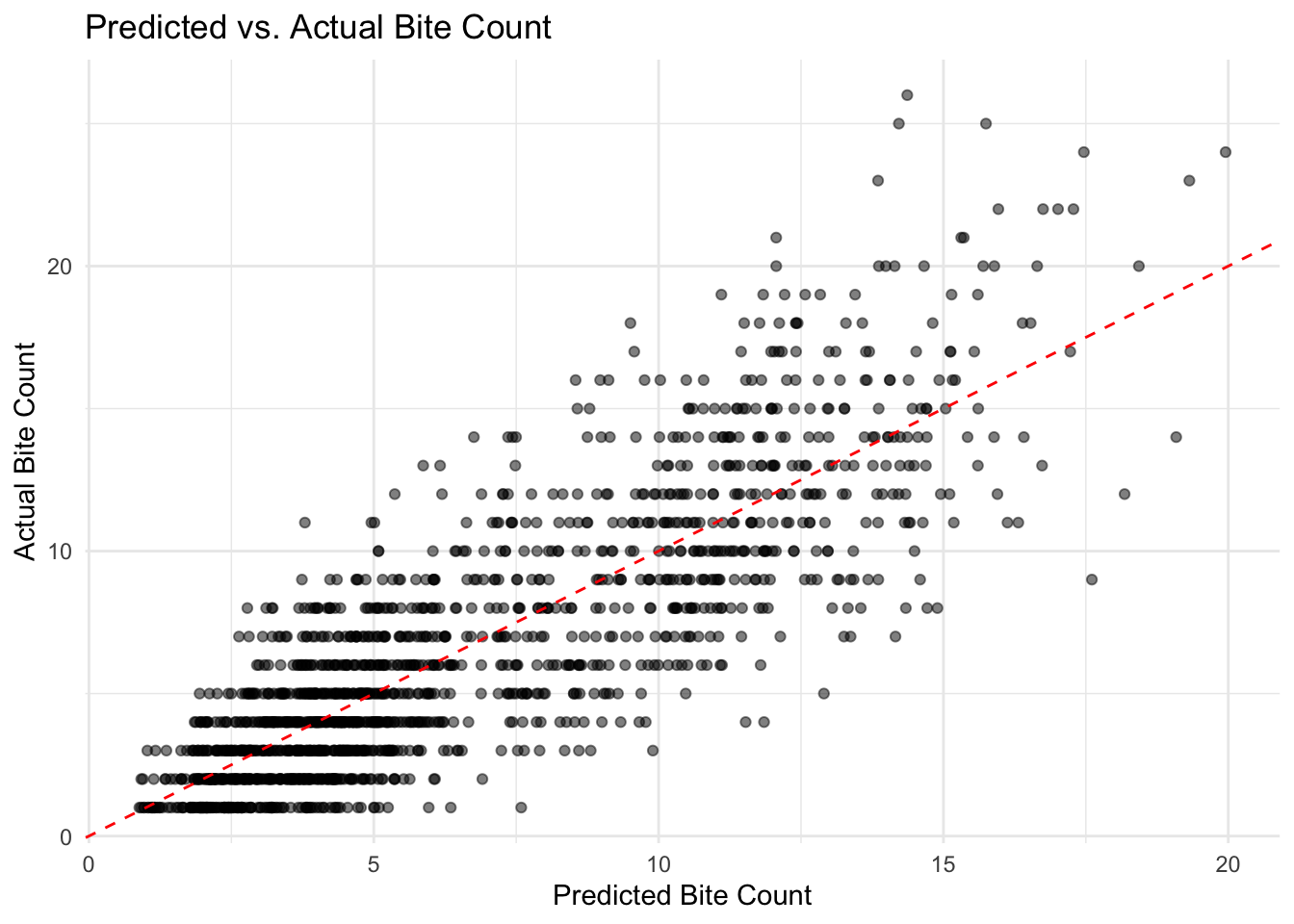
Cross-validation of the final model is depicted in the following
illustration, where the red dashed line represents the ideal prediction
scenario (i.e., predicted values equal actual values). If points fall
near this line, it indicates that the model predicts well. Points
located above the diagonal line suggest that the model underestimates
the actual values; conversely, if points are below the diagonal line,
the model overestimates the actual values.
# Predicted vs Actual Bite Count
inter_predict = bites_by_group |>
  mutate(predicted = predict(model_stepwise, type = "response"))

ggplot(inter_predict, aes(x = predicted, y = bite_count)) +
  geom_point(alpha = 0.5) +
  geom_abline(slope = 1, intercept = 0, color = "red", linetype = "dashed") +
  labs(title = "Predicted vs. Actual Bite Count",
       x = "Predicted Bite Count",
       y = "Actual Bite Count") +
  theme_minimal()

Overall, while the scatter plot shows a slight systematic deviation,
the final negative binomial regression model still accurately predicts
low and medium value areas. However, the error is larger in high-value
areas, where actual values tend to fall below the predicted values. This
may indicate a tendency of the model to overfit in regions with high
incident counts.
Generalized Linear Mixed Model (GLMM)
To address the model fitting issue, a generalized linear mixed model
is employed. The Generalized Linear Mixed Model (GLMM) is an extension
of the Generalized Linear Model (GLM) and the Linear Mixed Model (LMM).
GLMM consists of three main components: random effects, fixed effects,
and a link function. Fixed effects represent the overall level
parameters consistent across all observations, while random effects
account for individual variability or group-level differences that may
influence the response variable. The link function connects the linear
predictor to the mean of the response variable distribution, allowing
the dependent variable to deviate from a normal distribution and
enabling modeling of various types of data, including binary, count, and
continuous outcomes.
Let the response variable \(y\)
belongs to the exponential family, its conditional distribution can be
expressed as follows:
\[
f(y|b) = \prod_{i=1}^n f(y_i|\eta_i)
\]
Where \({\eta _i} = {x_i}^ \top \beta +
{z_i}^ \top b\). Additionally, the random effect \(b\) is assumed to be distributed according
to \(b \sim {\rm N}(0,\Sigma )\).
Therefore the GLMM is structured as follows:
\[
g(\mathbf{E}(y)) = \mathbf{X}\vec{\beta} + \mathbf{Z}\vec{b} +
\varepsilon
\]
In the model, \(g( \cdot )\)
represents the link function, which connects the expected value of the
response variable to the linear predictor. Here, the logarithm function
\(g(\mu ) = \ln (\mu )\) is used, which
is appropriate for the Poisson distribution. \(\vec{\mathrm{E}}(y)\) denotes the vector of
expected values for the response variable, and \(\varepsilon\) represents the error term,
capturing random noise or the unexplained variance. \({\rm X}\vec \beta + {\rm Z}\vec b\)
represents the linear combination of fixed and random effects, \({\rm X}\vec \beta\) is used to explain
global trends, and \({\rm Z}\vec b\) is
utilized to capture differences among observations. In this context,
\({\rm X}\) is the design matrix for
fixed effects, which is of order \(n \times
p\), where \(n\) is the number
of observations and \(p\) is the number
of fixed effect variables; \(\vec
\beta\) is the vector of coefficients for fixed effects, with
each element representing the regression coefficient of a fixed effect
variable. Similarly, \({\rm Z}\) also
serves as the design matrix for random effects, of order \(n \times q\), where \(q\) is the number of random effect
variables. \(\vec b\) is the vector of
coefficients for random effects, representing inter-group deviations
used to explain random differences between groups. The model assumes
\(b \sim {\rm N}(0,\Sigma )\), thereby
the random effects are normally distributed with a mean of \(0\) and a covariance matrix \(\Sigma\).
For the dog bite incidents dataset, the response variable \(y\) represents the number of dog bite
incidents per zipcode per month. Fixed effects in the model include
year, month, gender, and sterilization status. Random effects are
attributed to different boroughs (5 boroughs in total). Thus, for all
response variables, \({\rm X}\) is a
matrix containing year, month, gender, and sterilization status; \(\vec \beta\) represents the coefficients
for the fixed effects; \({\rm X}\)
indicates the matrix for the borough each response variable belongs to;
and \(\vec b\) denotes the deviation
for each borough (random effects). This setup allows the model to adjust
for the influence of both environmental conditions and borough-specific
variations in the occurrence of dog bites.
Results
glmm_model = glmer.nb(
  bite_count ~ year + month + gender + spay_neuter + (1 | borough),
  data = bites_by_group
)
summary(glmm_model)
glmm_model_summary <-
  broom.mixed::tidy(glmm_model) %>%
  mutate(
    significance = case_when(
      p.value < 0.001 ~ "***",
      p.value < 0.01 ~ "**",
      p.value < 0.05 ~ "*",
      TRUE ~ ""
    )
  ) |>
  dplyr::select(-effect, -group)

kable(
  glmm_model_summary,
  col.names = c("Term", "Estimate", "SE", "Statistic", "P-value", "Significance"),
  caption = "Summary of Negative Binomial Regression Results"
) %>%
  kable_styling(bootstrap_options = c("striped", "hover", "condensed"), full_width = TRUE) %>%
  scroll_box(height = "400px")
Summary of Negative Binomial Regression Results
|
Term
|
Estimate
|
SE
|
Statistic
|
P-value
|
Significance
|
|
(Intercept)
|
1.1804665
|
0.1699854
|
6.9445164
|
0.0000000
|
***
|
|
year2016
|
0.0698070
|
0.0416932
|
1.6743026
|
0.0940711
|
|
|
year2017
|
0.1535296
|
0.0409953
|
3.7450517
|
0.0001804
|
***
|
|
year2018
|
0.0752759
|
0.0416131
|
1.8089477
|
0.0704591
|
|
|
year2019
|
0.0941456
|
0.0414242
|
2.2727192
|
0.0230431
|
|
|
year2020
|
-0.2788938
|
0.0455420
|
-6.1238848
|
0.0000000
|
***
|
|
year2021
|
-0.2868691
|
0.0459453
|
-6.2437123
|
0.0000000
|
***
|
|
month2
|
0.0024859
|
0.0588592
|
0.0422342
|
0.9663120
|
|
|
month3
|
0.0299497
|
0.0584208
|
0.5126548
|
0.6081928
|
|
|
month4
|
0.1274342
|
0.0572598
|
2.2255456
|
0.0260446
|
|
|
month5
|
0.1806481
|
0.0567229
|
3.1847452
|
0.0014488
|
**
|
|
month6
|
0.2446528
|
0.0560720
|
4.3631934
|
0.0000128
|
***
|
|
month7
|
0.2018245
|
0.0566339
|
3.5636679
|
0.0003657
|
***
|
|
month8
|
0.2276003
|
0.0564774
|
4.0299325
|
0.0000558
|
***
|
|
month9
|
0.1429054
|
0.0572333
|
2.4968912
|
0.0125287
|
|
|
month10
|
0.0911307
|
0.0578934
|
1.5741114
|
0.1154617
|
|
|
month11
|
0.0889304
|
0.0579177
|
1.5354601
|
0.1246709
|
|
|
month12
|
0.0184990
|
0.0590100
|
0.3134894
|
0.7539089
|
|
|
genderM
|
0.8848816
|
0.0245647
|
36.0225275
|
0.0000000
|
***
|
|
spay_neuterNeutered
|
-0.1123005
|
0.0229100
|
-4.9018117
|
0.0000009
|
***
|
|
sd__(Intercept)
|
0.3600968
|
NA
|
NA
|
NA
|
|
Random Effects:
Borough: Variance: 0.1297, standard Deviation: 0.3601.
Indicates moderate variability between boroughs in the baseline bite
count.
Fixed Effects:
Year: 2017 has positive coefficient
(0.15336, p < 0.001), suggesting a higher bite count compared to
2015. While 2020 and 2021 have strong negative
coefficients (-0.27884 and -0.28669, p < 0.001), indicating a
substantial reduction in bite counts. This could relate to external
factors like the COVID-19 pandemic.Month: Positive coefficient (0.12734, p = 0.026),
suggesting higher bite counts in April. In May, June and July, all p
< 0.001, maybe there is a seasonal peak during summer.Gender: Male dogs have strong positive coefficient
(0.88482, p < 0.001), indicating male dogs have a significantly
higher bite count compared to female dogs.Spay/Neuter Status: Dogs who are neutered have have
significantly lower bite counts (-0.11231, p < 0.001).
Evaluation
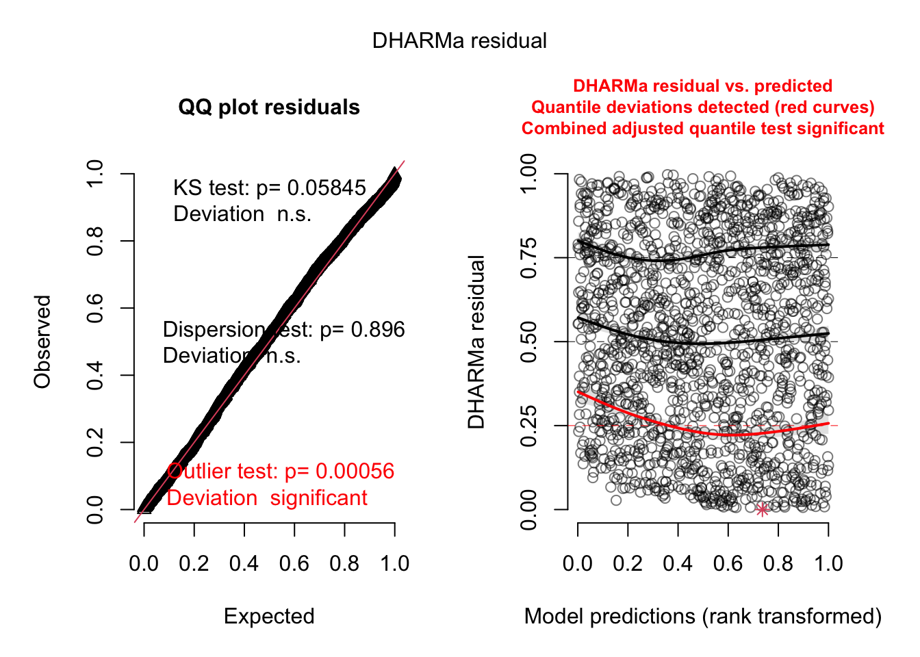
residuals_glmm_sim = simulateResiduals(glmm_model)
plot(residuals_glmm_sim)

Q-Q Plot:
- Kolmogorov-Smirnov (KS) Test: p-value = 0.05845: Indicates that the
residual distribution is not significantly different from the expected
distribution (n.s. means not significant). The model fits the overall
data distribution well.
- Dispersion Test: p-value = 0.896: Suggests no evidence of
overdispersion or underdispersion in the residuals. This confirms the
appropriateness of using the negative binomial model for handling count
data with dispersion.
- Outlier Test: p-value = 0.00056: Indicates significant deviations
due to outliers. This suggests that there are specific data points that
the model fails to fit well.
Residuals vs. Predicted:
- The red lines (quantile deviations) highlight significant deviations
at certain ranges of predictions, particularly near the lower predicted
values (around the 0.25 quantile). This indicates a slight mismatch
between the model predictions and observed data for certain ranges.
- Despite the overall good fit, systematic patterns (e.g., slight
curvature) in the residuals suggest possible room for improvement in
model specification.
Model comparison
model_comparison <- data.frame(
  Model = c("model", "filter_model", "glmm_model"),
  AIC = c(7403.4, 7045.8, 7428.7),
  Null_Deviance = c(3914.5, 4944.9, NA),
  Residual_Deviance = c(1549.7, 1437.1, 1551),
  Random_Effects = c("None", "None", "Borough"),
  Description = c(
    "Negative binomial regression with main effects only",
    "Negative binomial regression with main effects and interaction terms",
    "Negative binomial mixed model with random intercept for Borough"
  )
)

model_comparison %>%
  kbl(
    caption = "Model Comparison Table",
    align = "lcccccc",
    col.names = c("Model", "AIC", "Null Deviance",
                  "Residual Deviance", "Random Effects", "Description")
  ) %>%
  kable_styling(
    bootstrap_options = c("striped", "hover", "condensed", "responsive"),
    full_width = TRUE
  )
Model Comparison Table
|
Model
|
AIC
|
Null Deviance
|
Residual Deviance
|
Random Effects
|
Description
|
|
model
|
7403.4
|
3914.5
|
1549.7
|
None
|
Negative binomial regression with main effects only
|
|
filter_model
|
7045.8
|
4944.9
|
1437.1
|
None
|
Negative binomial regression with main effects and interaction terms
|
|
glmm_model
|
7428.7
|
NA
|
1551.0
|
Borough
|
Negative binomial mixed model with random intercept for Borough
|
Performance:
The filter_model has the lowest AIC and Residual
Deviance, suggesting the best fit among the three. However, its lack of
random effects might overlook some unobserved variability (e.g., between
boroughs).
Complexity:
glmm_model introduces random effects, which makes it
more flexible and suitable for accounting for regional differences, but
this increases its AIC and Residual Deviance slightly.
Interpretability:
model is the simplest and easiest to interpret but
underperforms compared to the other two models.
Residual Diagnosis:
model VS glmm_model: The KS test and
dispersion test results in both models are similar, suggesting both
models handle overall distribution and dispersion well. However, the
outlier test is significant in glmm model, whlie the
outlier test is insignificant in the model, indicating that
this alternative model has difficulty capturing certain extreme values
or specific subsets of the data.
